
통계 데이터 분석 -확률PYTHON/데이터분석2023. 9. 15. 17:16
Table of Contents
import enum, random
class Coin(enum.Enum):
  FRONT = 0 #앞면
  BACK = 1 #뒷면
  def random_coin(): #랜덤
    return random.choice([Coin.FRONT, Coin.BACK])

#------------------------------------------------------------

for _ in range(20): #20번
  if Coin.random_coin() == Coin.FRONT:
    print(".", end=' ') #앞쪽이면 .출력
  else:
    print("1", end=' ') #뒤면 1

    """
    . 1 1 . 1 . . . 1 . 1 . 1 1 1 . 1 . . 1

    """
만약에 동전을 두 번 던졌을 때 P(both|first)와 P(both|either)를 구하시오.
P(both|first) 첫 번째 던졌을 때 뒷면이 나오고 둘 다 뒷면이 나올 확률
P(both|either) 둘 중 하나가 뒷면이 나오고 둘 다 뒷면이 나올 확률
both_back = 0 #둘 다 뒷면이 나온 횟수
first_back = 0 #첫 번째 뒷면이 나온 횟수
either_back = 0 #둘 중 하나는 뒷면이 나온 횟수


for _ in range(10000):
  first = Coin.random_coin()
  second = Coin.random_coin()

  # if문으로 +1
  if first == Coin.BACK:
    first_back +=1
  if first==Coin.BACK and second == Coin.BACK:
    both_back+=1
  if first==Coin.BACK or second == Coin.BACK:
    either_back+=1

#확률출력
print("P(both|first)",both_back/first_back)
print("P(both|either)",both_back/either_back)


"""
P(both|first) 0.49779116465863454
P(both|either) 0.3310630341880342
"""
균등 분포
분포가 특정 범위 내에서 균등하게 나타나 있을 경우
누적 분포
주어진 확률 변수가 특정 값보다 작거나 같은 확률을 나타내는 함수
def uniform_pdf(x): #균등분포
  if 0<=x<1:
    return 1
  return 0
def uniform_cdf(x): #누적 분포
if x<0:
return 0
if x<1:
return x
return 1xs = []
pys=[]
cys=[]
#-1~2까지 step=0.01로 균등 분포와 누적 분포를 계산하여 컬렉션에 보관
for x_100 in range(-100,200):
pys.append(uniform_pdf(x_100/100))
cys.append(uniform_cdf(x_100/100))
xs.append(x_100/100)import matplotlib.pyplot as plt
fig, ax = plt.subplots(1,2) #여러 개의 그래프를 하나의 그림에 나타낸다.
# nrows=1, ncols=2, index
ax[0].plot(xs, pys, "b.", label="pdf")
ax[1].plot(xs, cys, "r.", label="cdf")
ax[0].set_title("The uniform pdf")
ax[1].set_title("The uniform cdf")
plt.show()
정규분포

#정규분포 식 표현
import math
SQRT_TWO_PI = math.sqrt(2*math.pi)
def normal_pdf(x, mu=0, sigma = 1): #정규분포 (mu:평균, sigma:표준편차)
  pre = 1/(sigma*SQRT_TWO_PI)
  post = math.exp(-((-x-mu)**2)/(2*(sigma**2)))
  return pre * post
xs = [x/10.0 for x in range(-50,50)]
ys1 = [normal_pdf(x, sigma=1) for x in xs]
ys2 = [normal_pdf(x, sigma=2) for x in xs]
ys3 = [normal_pdf(x, sigma=0.5) for x in xs]
ys4 = [normal_pdf(x, mu=1) for x in xs]
plt.plot(xs,ys1,'-', label="mu=0, sigma=1")
plt.plot(xs,ys2,'--', label="mu=0, sigma=2")
plt.plot(xs,ys3,':', label="mu=0, sigma=0.5")
plt.plot(xs,ys4,'-.', label="mu=1, sigma=1")
plt.legend()
plt.show()
정규누적분포

def normal_cdf(x, mu=0, sigma=1): #정규누적분포
  return (1+math.erf((x-mu)/(sigma*math.sqrt(2))))/2
xs = [x/10.0 for x in range(-50,50)]
ys1 = [normal_cdf(x, sigma=1) for x in xs]
ys2 = [normal_cdf(x, sigma=2) for x in xs]
ys3 = [normal_cdf(x, sigma=0.5) for x in xs]
ys4 = [normal_cdf(x, mu=1) for x in xs]
plt.plot(xs,ys1,'-', label="mu=0, sigma=1")
plt.plot(xs,ys2,'--', label="mu=0, sigma=2")
plt.plot(xs,ys3,':', label="mu=0, sigma=0.5")
plt.plot(xs,ys4,'-.', label="mu=1, sigma=1")
plt.legend()
plt.show()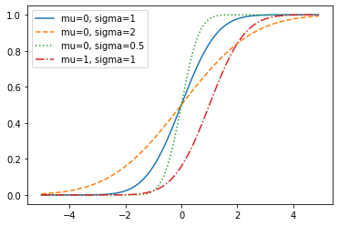
베르누이 시행
확률론과 통계학에서 임의의 결과가 '성공' 또는 '실패'의 두 가지 중 하나인 실험을 뜻한다. 다시 말해 '예' 또는 '아니오' 중 하나의 결과를 낳는 실험을 말한다.
#랜덤으로 수 뽑는 함수 만듬
def bernouli_trial(p):
  return 1 if random.random()<p else 0
cnt=0
for _ in range(100):
re = bernouli_trial(1/6)
print(re, end= '.') #확률이 1/6인 사건이 발생하면 1, 발생하지 않으면 0 출력
if re == 1:
cnt+=1
print()
print(cnt)
"""
1.1.0.0.0.1.0.0.0.0.0.1.1.0.0.0.0.0.1.0.0.0.0.0.0.0.0.0.0.1.0.0.0.1.0.0.0.0.1.0.0.0.0.0.0.1.0.0.0.0.0.0.0.0.0.0.0.1.0.0.0.0.0.0.0.1.0.0.1.1.0.0.1.0.0.0.0.0.0.0.0.1.0.1.0.0.1.1.0.0.0.0.0.0.0.0.0.0.0.0.
19
"""
def binomial(n,p):
  return sum(bernouli_trial(p) for _ in range(n))
for _ in range(20):
  print(binomial(100, 1/6), end='.') #주사위를 100번 던졌을 때 숫자 1이 나올 횟수

"""
16.24.21.12.18.22.12.19.18.13.14.14.21.17.16.18.20.29.11.17.

"""
from collections import Counter


def binomial_histogram(p,n,nps): # p:확률, n:시도할 횟수, nps:(p,n)을 시도할 횟수
  data = [binomial(n,p) for _ in range(nps)]
  histogram = Counter(data)
  mu = p*n
  sigma=math.sqrt(n*p*(1-p))
  xs=range(min(data), max(data)+1)

  #nomal_cdf에서 (i-0.5) ~ (i+0.5)의 변화량
  ys = [normal_cdf(i+0.5, mu, sigma)-normal_cdf(i-0.5,mu,sigma) for i in xs]
  ys2=[normal_cdf(i, mu, sigma) for i in xs]

  plt.bar(histogram.keys(),[v/nps for v in histogram.values()],color='r')
  plt.plot(xs,ys)
  plt.title("Binomial Distribution and Normal Approximation") #이항 분포와 정규 근사
  plt.show()


binomial_histogram(1/6, 100, 1200)
주사위를 100번 던졌을 때 1이 나오는 횟수가 40~60일 확률은 얼마인가?
p=1/6 #주사위
n=100 #100번던진다.
mu = p*n #평균(기대값)
sigma = math.sqrt(n*p*(1-p))
c1 = normal_pdf(13, mu=mu, sigma=sigma)
c2 = normal_pdf(18, mu=mu, sigma=sigma)

print(c1, c2)
print(c2-c1)

xs = [x for x in range(101)]
ys = [normal_cdf(x,mu=mu,sigma=sigma) for x in xs]
plt.plot(xs,ys)
x>5 일 때 99.7% 확률로 1
2x가 2보다 큰 수일 때 90% 확률로 1
0<x<=2 일 때 70% 확률로 1
x<=0일 때 0% 확률로 1
xs = np.arange(-10,10,0.3)
ys1=[]
for x in xs:
  if x>5:
    if np.random.uniform(0,10)>0.03: #0~10 사이의 랜덤한 수가 0.03 보다 크면
      ys1.append(1)
    else:
     ys1.append(0)
  elif x>2:
    if np.random.uniform(0,10)>1:
      ys1.append(1)
    else:
      ys1.append(0)
  elif x>0:
    if np.random.uniform(0,10)>3:
      ys1.append(1)
    else:
      ys1.append(0)
  else:
    ys1.append(0)


plt.plot(xs,ys1,'.')
plt.show()
'PYTHON > 데이터분석' 카테고리의 다른 글
| 1-3 마켓과 머신러닝 (0) | 2023.09.15 |
|---|---|
| 통계 데이터 분석 -KNN회귀 (0) | 2023.09.15 |
| 통계 데이터 분석 -선형회귀 (0) | 2023.09.15 |
| 데이터 분석에 자주 사용하는 문법 (0) | 2023.09.15 |
| 통계분석시각화 - 통합 (1) | 2023.09.15 |


