
통계분석시각화 - 통합PYTHON/데이터분석2023. 9. 15. 17:15
Table of Contents
!! 코랩 폰트설치!!
!sudo apt-get install -y fonts-nanum
!sudo fc-cache -fv
!rm ~/.cache/matplotlib -rf


"""
Reading package lists... Done
Building dependency tree
Reading state information... Done
fonts-nanum is already the newest version (20170925-1).
The following package was automatically installed and is no longer required:
  libnvidia-common-470
Use 'sudo apt autoremove' to remove it.
0 upgraded, 0 newly installed, 0 to remove and 39 not upgraded.
/usr/share/fonts: caching, new cache contents: 0 fonts, 1 dirs
/usr/share/fonts/truetype: caching, new cache contents: 0 fonts, 3 dirs
/usr/share/fonts/truetype/humor-sans: caching, new cache contents: 1 fonts, 0 dirs
/usr/share/fonts/truetype/liberation: caching, new cache contents: 16 fonts, 0 dirs
/usr/share/fonts/truetype/nanum: caching, new cache contents: 10 fonts, 0 dirs
/usr/local/share/fonts: caching, new cache contents: 0 fonts, 0 dirs
/root/.local/share/fonts: skipping, no such directory
/root/.fonts: skipping, no such directory
/var/cache/fontconfig: cleaning cache directory
/root/.cache/fontconfig: not cleaning non-existent cache directory
/root/.fontconfig: not cleaning non-existent cache directory
fc-cache: succeeded


"""
plt.rc('font',family='NanumBarunGothic')
실습코드
import pandas as pd
import numpy as np
import matplotlib.pyplot as plt

path = '/content/sample_data/train_titanic.csv'
df = pd.read_csv(path)
df
s1= pd.Series([1,2,3,4,5,6,10])
s1

"""
왼: 인덱스 오 : 값
0     1
1     2
2     3
3     4
4     5
5     6
6    10
dtype: int64

"""
s1.plot() #리스트의 값들이 y 값들이라고 가정하고, x 값을 자동으로 만들어낸다
plt.show()

df.Age.plot()
plt.title("Age")
plt.show()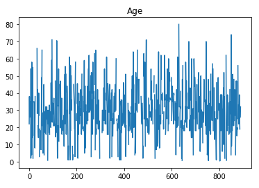
s2 = pd.Series([1,2,3,4,5,6,7,10], index=pd.date_range('2019-01-01' , periods=8))
s2

"""
2019-01-01     1
2019-01-02     2
2019-01-03     3
2019-01-04     4
2019-01-05     5
2019-01-06     6
2019-01-07     7
2019-01-08    10
Freq: D, dtype: int64

"""
s2.plot(grid=True)
plt.show()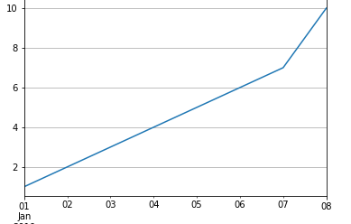
#파일읽어오기
df_rain = pd.read_csv('/content/sample_data/sea_rain.csv')
df_rain
df_rain2 = df_rain[['동해','남해','서해','전체']]
df_rain2.index=["1996","1997","1998"]
df_rain2

df_rain2.plot()
plt.show()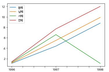
df_rain2.plot(grid=True , style=['r-*','g-o','b:*','m-.p'])
plt.xlabel('연도')
plt.ylabel('강수량')
plt.title("연간 강수량")
plt.show()

year =[2006,2008,2010,2012,2014,2016] #연도
area =[26.2,27.8,28.5,31.7,33.5,33.2] #1인당 주거 면적
table = {"연도" : year, "주거면적" : area}
df_area = pd.DataFrame(table,columns = ["연도","주거면적"])
df_area
df_area.plot(x="연도" , y="주거면적", grid=True ,title="연도별 1인당 주거면적")
plt.show()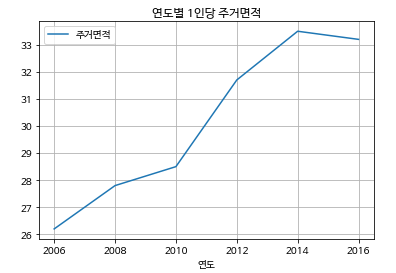
df.plot("PassengerId" , y="Age" ,grid=True ,title="승객나이")
plt.xlabel("승객 id")
plt.ylabel("나이")
plt.show()

#산점도
temperature = [25.2,27.4,22.9,26.2,29.5,33.1,30.4,36.1,34.3,29.1]
sales = [236500,357500,203500,365200,446600,574200,453200,675400,598400,463100]
dict_data = {"기온":temperature,"판매량":sales}
df_sales = pd.DataFrame(dict_data,columns=["기온","판매량"])
df_sales
df_sales.plot.scatter(x='기온',y='판매량',grid=True,title="온도와 판매량")
plt.show()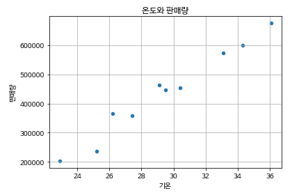
#막대그래프
grade_num =[5,4,12,3]
students=["A","B","C","D"]
df_grade = pd.DataFrame(grade_num , index=students ,columns=['Student'])
df_grade
df_grade.plot.bar()
plt.xlabel('학점')
plt.ylabel('학생 수')
plt.title("학점 별 학생 수 그래프")
plt.show()
#히스토그램
어떠한 변수에 대해서 구간별 빈도수를 나타낸 그래프
bin : 구간(막대갯수)
math=[90,85,75,70,77,80,85,87,89,90,60,87,75]
df_math = pd.DataFrame(math, columns=['Student'])
df_math.plot.hist(bins=8 ,grid=True)
plt.xlabel('시험 성적')
plt.ylabel('도수')
plt.show()
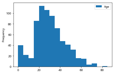
adf = df[['Age']] #데이터 프레임
adf.plot.hist(bins=[age for age in range(0,86,5)])
plt.show()
#파이그래프
fruit=['사과','바나나','딸기']
result =[7,6,3]
df_fruit = pd.Series(result, index=fruit , name ="선택한 학생 수")
df_fruit

"""
사과     7
바나나    6
딸기     3
Name: 선택한 학생 수, dtype: int64
"""
df_fruit.plot.pie()
plt.show()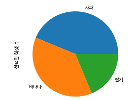
'PYTHON > 데이터분석' 카테고리의 다른 글
| 통계 데이터 분석 -선형회귀 (0) | 2023.09.15 |
|---|---|
| 데이터 분석에 자주 사용하는 문법 (0) | 2023.09.15 |
| 통계분석시각화 - 타이타닉2 (0) | 2023.09.15 |
| 통계분석시각화 - 타이타닉1 (0) | 2023.09.15 |
| 통계분석시각화 : matplotlib (1) | 2023.09.15 |


